In this article , we get our hands dirty with very basic linear regression using recent version of tensorflow. Linear regression is usually considered as first baby step in the algorithms world.
What Is Linear Regression ?
- Linear regression in easy terms is a straight line passing nearby to all the data points we plot.
- Technically , Linear regression gets us the relationship between one or more variable(s) . Linear regression is a first step for all ML enthusiasts and used for predictive analysis and modelling.
- Our teacher once a time said , y=mx+b is a linear equation & it stands true even today.
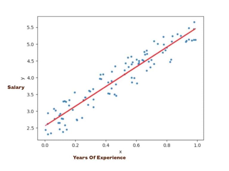
- Given below is a linear regression graph between years of exp. vs salary. Say we want to predict X = 1.2. We can just extend the read line & get the value at that moment.

Some Facts About Linear Regression
- Major types of regressions include Linear Regression , Polynomial Regression , Ridge Regression , Lasso Regression.
- Except Linear Regression , rest of the types are well suited for higher dimensions data analysis.
- Linear regression is a great way start to the journey of machine learning as it is quite straightforward and your first step for using models in machine learning world.
How can we implement linear regression from scratch?
- Assume x is the feature and y is target ( y = mx + c)
- In order to find the value of m and c, you first need to calculate the mean of x and y
Algorithm below :
Step 0 : calculate the mean of x and y
Step 1 : total number of reccords
n = len(x)Step 2: Use these steps to calculate m and c.
( Bascially we are capturing the distance of a point from its mean )
numerator = 0denominator = 0for i in range(n):numerator += (X[i] - mean_x) * (Y[i] - mean_y)denominator += (X[i] - mean_x) ** 2
Step 3: m = numerator / denominator
Step 4: c= mean of y - (m * mean of x)
So we now have m and c. Which we can use to do further predictions!
Where can we use Linear Regression ?
- Estimating price of a house after 2 years.
- Predicting value of a share of 5 years
- Predicting amount of rainfall for coming days.
And many more places where we want to forecast a continuous value.
Here we are implementing a linear regressor using tensorflow with manually created data.
Before we begin , Some prerequisites !
Before we begin , Some prerequisites !
| Python Version | Difficulty Level | Pre-Requisites |
| 2.7+ | Easy | Basic Python |
Download the input file from THIS LINK.
”’
Import Modules
”’
import tensorflow as tf
import numpy as np
import pandas as pd
import matplotlib.pyplot as plt
%matplotlib inline
”’
Read the data into datafames
File has 2 colums. 1 : Year & 2 : Value
”’
df = pd.read_csv(‘sample_file.csv’, header=None)
# Make X a 2-D array of size N x D where D = 1 / .values converts series to numpy arrray
X = df.values[:,0] #.reshape(-1, 1)
Y = df.values[:,1]
”’
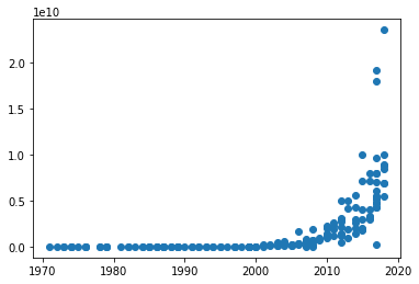
Plot the data – it is exponential
”’
plt.scatter(X, Y)

# Since we want a linear model, we take the log
Y = np.log(Y)
plt.scatter(X, Y)

”’
Remember to scale the data
”’
X = X – X.mean()
”’
Let’s create a TensorFlow model structure here
”’
model = tf.keras.models.Sequential([
tf.keras.layers.Input(shape=(1,)),
tf.keras.layers.Dense(1)
])
”’
Compile the model
”’
model.compile(optimizer=tf.keras.optimizers.SGD(0.001, 0.9), loss=‘mse’)
”’
Set learrning rate
”’
def lean_rate(epoch, lr):
if epoch >= 50:
return 0.0001
else :
return 0.001
scheduler = tf.keras.callbacks.LearningRateScheduler(lean_rate)
”’
Train the model
”’
fit = model.fit(X, Y, epochs=200, callbacks=[scheduler])
Epoch 199/200 6/6 [==============================] - 0s 2ms/step - loss: 0.9062 - lr: 1.0000e-04 Epoch 200/200 6/6 [==============================] - 0s 2ms/step - loss: 0.8759 - lr: 1.0000e-04 ”’
Let’s Plot the results
”’
# Plot the loss
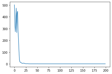
plt.plot(fit.history[‘loss’], label=‘loss’)

”’
our network has one layer only
Lets display value of m & b in linear equation y = mx + b
”’
print(model.layers)
print(model.layers[0].get_weights())
[] [array([[0.33869487]], dtype=float32), array([17.776506], dtype=float32)] Okay , Lets make predictions !
”’
We use same X to pedict
”’
pred = model.predict(X).flatten()
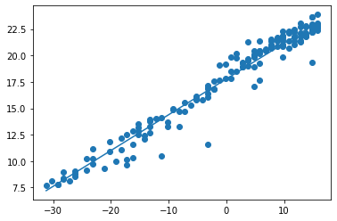
plt.scatter(X, Y)
plt.plot(X, pred)

”’
Let’s veify is our model accurate
”’
# We get the weight(w) and bias(b)
w, b = model.layers[0].get_weights()
#we apply y = mx + b
pred2 = (X.dot(w) + b).flatten()
# We check if output of pred(calculated by model) & pred2(manually pedicted) are close to each other
np.allclose(pred, pred2)
True
Wow , we built a basic linear regression using most recent version of TensorFlow.
You may like these recent heroics Below !