In this article , we implement Linear classification using most recent version of Tensorflow. i.e 2.2+
What Is Linear Classification ?
- When a data points to be classified are separable by a line or in easier terms we can draw a line between success records vs failure records , we call it Linear Classifier.
In the field of data science or machine learning , A linear classifier has a target of statistical classification to identify which output class an input set belongs to.
By using values of linear combinations and making a classification decision, a linear classifier achieves its end goal.
Examples of linear classifier include , Logistic Regression , NB classification etc.
What is the difference between linear and nonlinear classification techniques?
For 2D feature space, say data having only x-axis and y-axis. If one can draw a line between points without cutting any of them, they are linearly separable.
Now , look at the image below (on your right) . Such cases where data is not separable using a straight line falls under non-linear category. Here we needed aa circle to separate out the points.
Same goes for clusters in 3D data. Only difference being , A plane is used there instead of line.
This type of classifier works better when the problem is linear separable.

What is the difference types of linear classifiers ?
Majorly divided into :
A : Generative ( assumes conditional density functions ) :
A1 : Linear Discriminant Analysis (LDA)—assumes Gaussian conditional density models
A2 : Naive Bayes classifier with multinomial or multivariate Bernoulli models.
B : Discriminative models
(attempts to maximise the quality of the output on a training set)
B1 : Logistic regression
B1 : Perceptrons
B1 : Support Vector Machines(SVM)
- Following stunt shows us how can we implement a linear classier using very famous tensorflow libary.
- This code also demonstrates , how can we save the model and use it in production.
| Python Version | Difficulty Level | Pre-Requisites |
| 2.7+ | Easy | Basic Python |
(array(['malignant', 'benign'], dtype='<U9'), array(['mean radius', 'mean texture', 'mean perimeter', 'mean area', 'mean smoothness', 'mean compactness', 'mean concavity', 'mean concave points', 'mean symmetry', 'mean fractal dimension', 'radius error', 'texture error', 'perimeter error', 'area error', 'smoothness error', 'compactness error', 'concavity error', 'concave points error', 'symmetry error', 'fractal dimension error', 'worst radius', 'worst texture', 'worst perimeter', 'worst area', 'worst smoothness', 'worst compactness', 'worst concavity', 'worst concave points', 'worst symmetry', 'worst fractal dimension'], dtype='<U23'))
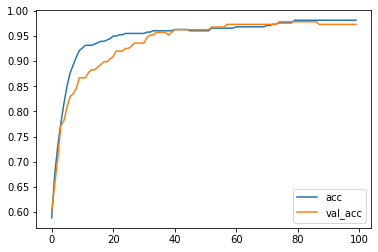
Epoch 100/100 12/12 [==============================] - 0s 4ms/step - loss: 0.0855 - accuracy: 0.9816 - val_loss: 0.1101 - val_accuracy: 0.9734 Test score: [0.10941322147846222, 0.9734042286872864] 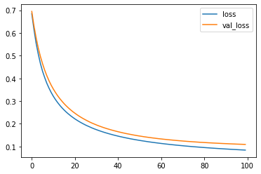
Lets use this model to make Predictions
Manually calculated accuracy: 0.973404255319149 6/6 [==============================] - 0s 2ms/step - loss: 0.1094 - accuracy: 0.9734 Evaluate output: [0.10941322147846222, 0.9734042286872864]
Lets save this model to deploy it in production
-rw-r--r-- 1 root root 18480 Jun 5 07:41 linearclassifier.h5 We can optimise this model to get better accuracy by chaging values like epochs,
number of hiddenn layers etc
[<tensorflow.python.keras.layers.core.Dense object at 0x7fd15925eb38>]
6/6 [==============================] - 0s 2ms/step - loss: 0.1094 - accuracy: 0.9734
[0.10941322147846222, 0.9734042286872864]