So you are here to take a risk of learning recurrent neural networks all by yourself. Appreciated ! When I first began my journey to understand recurrent neural networks ( RNNs ) , I honestly felt , Oh God ! save me 😀
This is my attempt to explain you recurrent neural nets in layman terms and as simple as possible so that you too don’t get that OMG feeling. This article will have recurrent neural networks explained in simple terms.
So let’s begin the journey which I call ” Recurrent neural nets in a nutshell ” 😛
Distraction Alert : If you are fascinated about computer vision and want to learn Convolutional neural networks in layman terms , phew ! you may read it here.
1.Why do we need recurrent neural nets ?
When we need algorithms to evaluate data in sequence/order we consider recurrent nets because normal artificial neural nets and convolutional neural nets love to evaluate data randomly.

If you guys know artificial neural nets(ANN) or Convolutional neural networks (CNN), whatever data you feed to the models, they don’t follow an order when been evaluated.
Confused ?
Lets make it simple.
Imagine 2 sentence ” I love scarlett johansson because she is beautiful ” & ” I love beautiful because she is scarlett johansson “.
Though the second sentence doesn’t make sense , when we feed this to a ANN or CNN the final output would be same as the position of words doesn’t matter to these algorithms.
Now imagine we see a beautiful girl and wanna propose her. Our sentence should come out in sequence as “I love you” and not in random. RNNs help in this case.
RNNs are best used in stock predictions , weather forecasting etc where our future forecasts are somewhat dependent on previous data.

2. ANNs Vs RNNs | What are recurrent neural nets ?
Recurrent neural nets are type of neural nets which were designed specially for those data whose future depends on their past.
2.0 ANN
Okay, so this is how a normal neural net looks like.
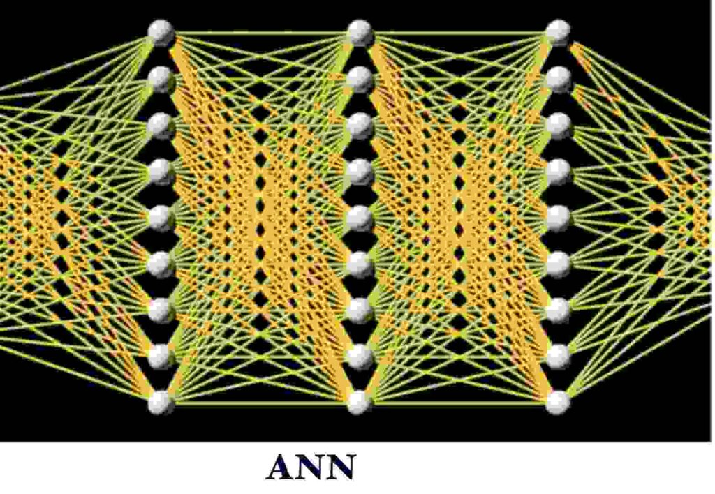
In a normal fully connected ANN We have an input layer , one or multiple hidden layers and one output layer.
Note : A neural network is called fully connected if all the nodes from one layer are connected to all the nodes of next layer.
Now lets take a look at one node layer.

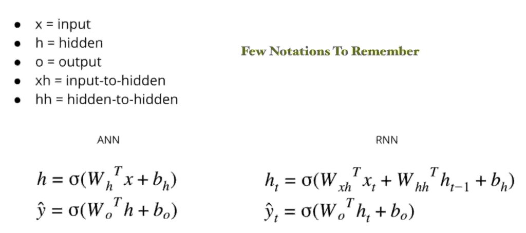
Consider x = input , h= hidden node , y = output node . The formulae for output calculations are as below.
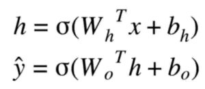
ANN formulae in words :
Hidden node output = activation function ( Weight of hidden node * input
PLUS
bias of hidden node )
Final Output = activation function ( Weight of output node * hidden node output
PLUS
bias of output node )
2.1 RNNs in detail
Time to get to the point , lets get started with RNNs !
Recurrent neural networks are similar to ones above but with one major difference. That is , it has a hidden node pointing to itself.
So , What does this mean? The following pic gives you a clear imagination.
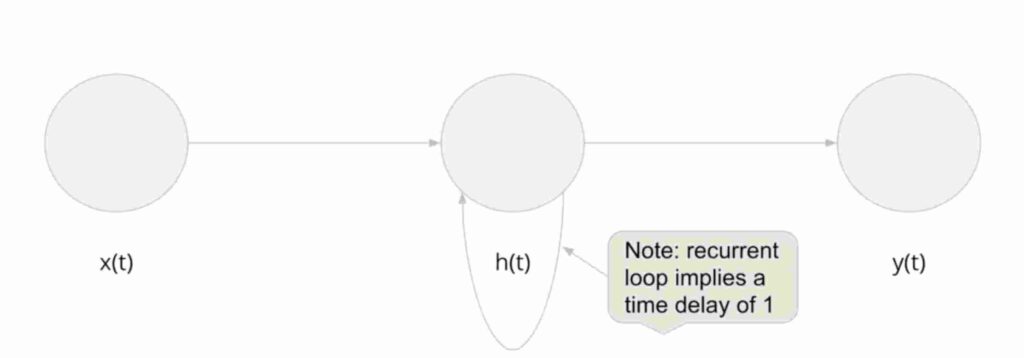
When we see ANN ONE NODE pic above , we see a slight difference. In RNNs , the previous state/value of the node contributes to the output of the hidden node.
Look at the formulae for calculations below. You will be much clearer !

Look at the highlighted in green section of the formulae. when comparison with normal ANN we see a h( t-1 ) in picture. In easy terms we can remember this as the output of hidden node is dependent on the previous value of hidden layer too.
Checkout text of formulae below to make it dead clear.
RNN formulae in words :
Hidden node output = activation function ( Weight of hidden node * input
PLUS
Weight of hidden to hidden node * State of hidden node at previous iteration
PLUS
bias of hidden node )
Final Output = activation function ( Weight of output node * hidden node output
PLUS
bias of output node )
If we want to understand what happens inside hidden layer in RNNs , it’s amazing to know that every hidden layer in RNN is a neural network in itself.
Don’t trust me ?
See an image of hidden layer of RNN unrolled.
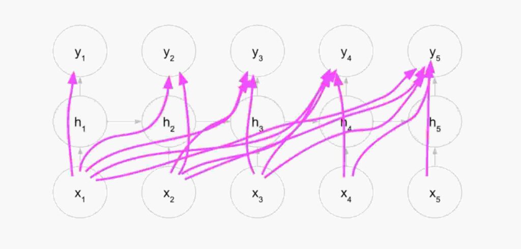
Well , don’t get freaked out with so many connections ! The pic just tells us that every next iteration inside a hidden layer of RNN will be dependent on values of previous iteration.
This means the final iteration h5 will depend on all previous iterations.
2.2 Few Important formulae to remember

3. Pseudocode of recurrent neural nets in Python
If all the above formulae scared you , then i’ve some relief for you. The actual code for RNNs is just few lines of program below.
The loop is a RNN in short.
Note : When it comes to RNNs , one has to always remember these notations.
At current times , all the work in the backend is done by libraries like keras ,pytorch. But its always good to understand how are these libraries built.
- N = number of samples
- T = sequence length
- D = number of input features
- M = number of hidden units
- K = number of output units
3.1 Simple RNN Code from scratch
h_last = np.zeros(M) #initial hidden state
x = [1,2,3,4,5] #Your innput
Yhats = [] # where we store the outputs

for t in range(T):
  #we calculate this as per RNN formulae we saw earlier
  h = np.tanh(x[t].dot(Wx) + h_last.dot(Wh) + bh)

  # Though we calculate this everytime , we only care about this value on the last iteration
  y = h.dot(Wo) + bo
  Yhats.append(y)

  # important: Assign h to h_last. This is where we loop hidden to hidden
  h_last = h

# print the final output
print(Yhats[-1])
3.2 Simple RNN using Tensorflow
Give above is a simple single input RNN code. But in real life if you want to write this using any modules , say tensorflow. We would just write :
M = 5 # number of hidden units
i = Input(shape=(T, D))
x = SimpleRNN(M)(i)
x = Dense(K)(x)
That’s crazy isn’t it ?
But the reality in data science & machine learning world in current generation is , you just have to know how to use the modules. Knowing the math behind them is great but that is often underestimated by any aspiring data scientist which one definitely shouldn’t.
4. Major drawbacks of RNNs & Origin of LSTM/GRUs
Now , consider the below wiki description and we have RNNs to build a question answer model.
RNN scans the words from beginning till the end and keeps updating weights ( h , h-1 , h-2 … h-n ).
When the training is over and RNN is at the end of the sentence , imagine we ask RNN ” what’s the birth date of Scarlett Johansson ? “.


The RNN will probably fail to answer as the date of birth is in the beginning of the paragraph and as RNN reaches the end updating weights i.e ( h , h-1 , h-2 … h-n ) , the first few iterations will not have a genuine weight. All thanks to a villain vanishing gradient problem !


Okay , there are many definitions of gradient problems but i’ll try to give you a simple intuition.
Checkout the image below.
4.1 What is vanishing gradient problem ?


Node 1 ( x1,h1,y1 ) would start reading the wiki paragraph. It would sequentially read as we humans do and when it completes reading , it would do 2 things.
One : Keep updating weights of previous weights of (h-1,h-2 .. )
Two : Continue reading the sentences.
It so happens weights of h1 , h2 , h3 aren’t updated enough to reflect the actual output. That mainly happens due to back propagation of updated weights using derivates of functions.
Sounds too technical ?
Okay , remember this as we have 10 chocolates and 7 students to share with. We keep giving two each from the end and by the time we reach kid 4-5 we realise there aren’t sufficient chocolates for everyone. Hence we keep giving 1 each from kid 5.
Though not spot on , this explanation tells us the distribution is not uniform for kid 1-7 with lesser resources available for kids in the beginning.
Same way , the initial layers in the neural network will not see a major change in weights therein not bringing in improvements in predictive ability of any neural network.
Refer this notebook for a practical demo by stanford university about gradient problems.
4.2 Emergence of LSTM & GRUs
Though usage of activation functions were suggested to reduce the gradient problems in ANNs , It didn’t work effectively in the RNNs. The main reason being the loopback to the current hidden node and considerations of time ( t-1 ) when calculating next values.
Here a decade old technique of LSTM & a modified version of GRUs came into picture. Lets understand how are LSTM & GRUs help managing gradient problems better.
5. LSTM & GRUs explained in layman terms
In case you get lost in any terms/explanation below , or you feel things are going over your head , Always remember one thing.
Every node/gate/junction/formulae you see in RNNs , their formulae or math finally has same structure i.e
output = activation_function( weights * input + ( weights * hidden_node -1 ) + bias)
In short , Check below.


You may just see difference in alphabets used in notation but trust me , each and every formulae below follow same structures.
LSTM Stands for Long Short Term Memory & GRU stands for Grated Recurrent Units.
Lets get started with GRUs and their math and simple explanations.
5.1 GRUs
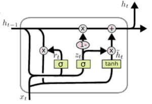

So don’t be freaked out with the james bond like diagram above.
Easy way to remember GRUs is , they have a memory gate for all things they do. A gate each to remember weights , forget weights and Reset weights.
Checkout the formulae below comparing how normal RNN calculations are done vs ones in GRUs. As I highlighted before, the structure remains the same.
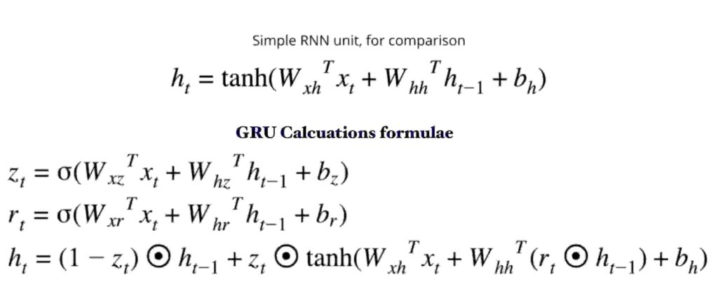

Again, one need not remember these equations. But let these thing be in your memory on how the above formulae works.
Checkout below for a quick easy breakup.


You would see , it’s that simple. The equation has a keep gate & a discard gate. Keep to continue placing a weight in the memory and discard to delete the unnecessary weights. Besides theres also a reset gate (check r in the equation to the right ) which resets weights when needed.
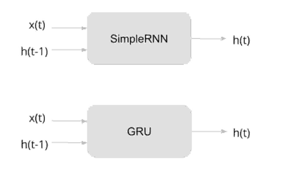
But end of the day , as a data scientist or for an ML engineer , when we implement RNNs or GRUs the structure remains same as below 😀

5.2 LSTMs
Firstly , the scary part ! How does a LSTM looks like ?
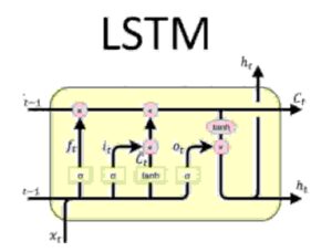

Don’t worry , even I couldn’t understand this at first go !
Pretty similar to GRUs , LSTM has just few features extra. Checkout the pic below.
We see a one extra c( t-1 ) in LSTMs. Thats nothing but self state. So , now the prediction not only depends on x(t) input & h( t-1 ) hidden state with time & also depends on c( t-1 ) self state.


So , besides these , LSTM has few same concepts of gates.
The gates function as below :
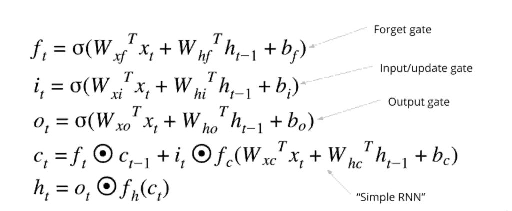

Remember , each gate has a specific job. The gate names says it all.
The major thing we got to understand is , the concept of GRU & LSTM came into picture because of vanishing gradient problem. i.e RNNs had difficulties to manage weights of every neurons. The concept of gates help manage weights affectively.
Forget gate , Input/Update gates , Output Gates all help to keep relevant weights & forget unimportant weights.
Refer this link for much more technical explanation on LSTMs & GRUs. My attempt is to explain concepts mostly in a non-technical and easy ways so that you go back with some learning and not just reading this article.
Tip to remember the math :
Checkout the pattern of every formulae above.
Everything resembles :
output = activation_function( weights * input + ( weights * hidden_node -1 ) + bias)
So , This should be a final view 🙂 I know this looks fancy and won’t help one understand anything. But i believe i’ve kept concepts as simple as possible in my post.


6. Final Say
Honestly , as a data scientist whatever you studied until now can be implemented in just these few lines of code below.
On a lighter note , even if 90% of the concepts you studied got over you , a few lines of code below can still make anyone a data scientist 😛
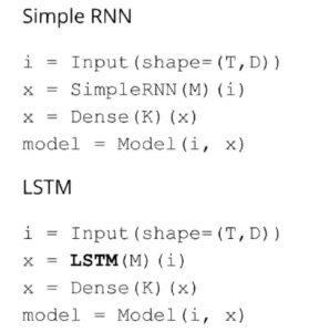

Concluding ,
We began with RNNs followed by how they work. Then the drawbacks and what made LSTMs and GRUs come into picture.
Assuming you learnt some amazing things about RNNs today , in case you are a beginner and felt like most of the concepts went over your head , Don’t worry !
It took me weeks of effort to understand RNNs and you may go through this article again after which i definitely feel you’ll catch things better.
A neural network learns better after many iterations , so as we 🙂
This was an attempt to explain things in layman terms and keep complexity as simple as possible.
Thanks for reading !
You may not want to miss these amazing articles !
- Hashing In Python From Scratch ( Code Included )

 We cover hashing in python from scratch. Data strutures like dictionary in python use underlying logic of hashing which we discuss in detail.
 - Recursion In Python With Examples | Memoization

 This article covers Recursion in Python and Memoization in Python. Recursion is explained with real world examples.
 - Unsupervised Text Classification In Python

 Unsupervised text classification using python using LDA ( Latent Derilicht Analysis ) & NMF ( Non-negative Matrix factorization )
 - Unsupervised Sentiment Analysis Using Python

 This artilce explains unsupervised sentiment analysis using python. Using NLTK VADER to perform sentiment analysis on non labelled data.
 - Data Structures In Python – Stacks , Queues & Deques

 Data structures series in python covering stacks in python , queues in python and deque in python with thier implementation from scratch.
