Hey Reader , I’m pretty sure you are itching to learn computer vision and here to get started with Convolution neural networks. I always dreamt of convolution neural networks (CNN) as very fancy. Maybe I was partly right. Today after knowing how they work , I sincerely feel one has to appreciate the thought behind this magic algorithm. This article tries to explain Convolutional neural networks in a simple and layman terms.
When tech world followed traditional ways to deal with visual data ( images, videos etc ) , Yann LeCun came up with a simple yet a revolutionary method for dealing with visuals. That’s convolution neural nets.
Lets jump into the journey of – “what i call a CNN nutshell” 😛
One secret trick to remember concepts in Data Science is to visualise the same in our mind.
1. Prerequisite to undertand CNNs

Okay ,That pic was just to show you what a convolution can do !
Don’t be tempted to scroll down assuming CNN explanation may get over your head. The prerequisite to understand this post is pretty basic.
Do you know addition & multiplication ? Hopefully yes , as you are here reading this article today 😀 .
If you want to understand convolutions , you just have to know 3 main things :
1 : Matrix & Its Operations like transform , reshape etc
2 : Addition.
3 : Multiplication.
Sounds easy ? Yes it is ! Using these 3 concepts and some real innovative thinking by Yann LeCun , We have an easy yet most reliable way of dealing with moving data today ! A live example of great things are built on simple basics yet highly effective.
So , if you have some idea on matrix , addition & multiplication we are good to proceed. If this doesn’t motivate you to continue , with convolutions one could accomplish photoshopping image transformations like one in pic above and definitely not limited to, but much more. So let’s begin!
2. What is a Convolution ?
Convolution in layman term is feature extraction on an image.
We apply so called a ‘filter‘ ( again a matrix ) on the image and pull out relevant features that makes sense for our predictions.

For a high school kid , we can say this as :
1 : We take an image , convert it into a matrix of pixels.
2 : Select a matrix ( randomly chosen ) of size say 2*2 or 3*3 and do a DOT product with output of 1 above.
That should be it. That’s convolutions in simple terms.
Just in case, you are wondering what are pixels , like how neurons are basic block of our brain , every image are made of bunch of pixels. Refer this link for an interestingly short yet a quick explanation on how are pixels and images related.
3. How does convolution work?
The images below speak a thousand words. As we discussed above , we take a matrix (called filter) and then multiply with images (converted to pixels). The output looks like one below.
Step one :
We pick up an image and convert it to matrix of pixels. & Next we pickup a filter. Here we take a 2*2 matrix.
Remember : There is no rule to select filter dimensions. It’s our guess which gets better with experience. But 2*2 or 3*3 matrix is generally preferred.

Step Two :
As promised before , We are multiplying & adding the filter with image. Observe the equation below for a clear understanding.

Step Three :
Continue this till the filter slides on the whole image.


We continue this till final slide.

In short :

4. Understand Shapes & A brisk CNN pseudo code
The major confusion everyone face in the convolution neural network world is the shape of matrices. The matrix has certain shape during input , gets changed to something else due to mathematical operations and when output they again change shapes.
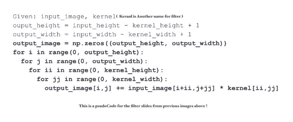
We know the input_height (No of rows in a matrix) & input_width (No of columns in a matrix). Besides these the major things to remember in ConV nets is the output_height & the output_width. This applies to the output to every layer involved in the network.

Given above is the pseudocode for a convolution operation. In short this code helps implement all the strides we see from a filter which is demonstrated in the images above. i.e They get us a dot product of matrices followed by addition.
In linear algebra , we can shorten above pseudocode as an equation below. This is good to understand but remembering the equation is not mandatory.

5. What is Padding ?
Most of the times we need input image size to be same as output image size. But when we apply a filter multiplication , we normally loose dimensions. You can see the output dimension in the gif image above where 5*5 matrix is reduced to 3*3.
To keep dimensions intact , i.e to keep input vs output dimensions as per user needs we use a concept of padding.
Another important place where padding helps is when we have images of uneven dimension. Lets say we have our childhood pics taken from different cameras and few are black and white and few colour. In order to do convolutions , we need to get it into a matrix of same dimensions. This is achieved by padding.

The white portion we see is padding. We usually do this by appending zeros to the matrix.
Note : Anything multiplied by zero is zero , so that won’t play a role or alter anything in the existing process of convolution.
In real world scenario, when we implement any convolutions using keras or tensorflow , we get this preloaded with a parameter named “mode“.

Of 3 values for mode above , following 2 are widely used.
1 : Valid – We don’t pad the input image with any zeros.
2 : Same – We pad enough zeros to the input image matrix to make input dimension same as output.
This is how ( 3 ) full padding looks like and is very rarely used. This results in a larger output image than a dimension of an input image.

In reality we have libraries which handles all these pad operations. We just have to know what can we use which gets us best results.
6.1D vs 2D vs 3D Convolutions
When dealing with 1D , 2D or 3D data , the only difference in convolutions is the shape of the input matrix followed by shape of filters which are adjusted accordingly as per dimensions.
Refer images below for a clear visuals.
So let’s talk about our daily activities. We listen to music , watch TV series , Netflix series , use smart watch during exercises etc etc.
So we are unknowingly dealing with all types of data everyday. i.e Signal of a smart watch – 1D data followed by black & white images – 2D data followed by coloured images – 3D data.
So , whats the difference between these 3 ? and how are convolutions different in 1D vs 2D vs 3D ?
Follow on for a visual understanding.

Image above explains a 1D filter slider ( on text data ) vs on a black and white image using a 2D filter slider. We observe the difference in sliding patterns , 1D slides in 1 direction followed by 2D which slides in 2 directions (moving Right followed by down )
Refer this link for an interestingly short yet a quick explanation on how images can be 2D or 3D based on certain features.


These quick visuals shows us how does the filters vary with data dimensions. This wraps up our first important concept of filters.
A quick takeaway : The dimensions of filters depend on the dimensions of input data we intend to convolve on.
7. What is Pooling ?
The second magic about CNN ( after filters ) is pooling. Pooling in simple terms means , Consider a matrix M.
We either take a max ( max pooling ) of M , min ( min pooling ) of M , average ( average pooling ) of M.
The concept is simple and straight forward yet very effective in retaining important information which matters to the final results.


Pooling helps us in 2 ways :
- Reduce the input dimension and keep only important features
- It helps identify an image irrespective of its position in an image.
Check the image below. Both the image are of alphabet ‘A‘. But ‘A‘ is not in same location. Pooling helps cover this up and yet identify where is the alphabet ‘A‘. This is a masterstroke as it helps identify any image irrespective of any position.

8. Complete end to end CNN

So we are almost there 🙂
- Convert the image into a matrix of pixels.
- Use filter matrix to create a dot product and convolve.
- Apply pooling ( sub sampling ) and experiment which works well. i.e max pool , avg pool etc.
- Create a fully connected dense layer ( where every input neuron is connected to every output neuron )
- This isn’t been covered in this article but you can refer this for more info.
- In layman term , fully connected layer ( also called dense layer ) has every input node having a connection to every output node of next layer.
- The final stage will be the output.
Note : Points 2 & 3 above can be repeated any number of times within the architecture. There is no ruleset asking us to use specific numbers but end of the day its all trail and error game. We need to trail error best architecture that gives us desired results.
In the diagram above steps 2 & 3 are repeated twice !

9. Final Take
Technology has come a long way since CNN were first used. Despite new findings , CNN remains a heartthrob even today for moving data ( audio , video ) analytics.
One final point i would like you to know is , in real world , modules like tensorflow , keras & pytorch gives us a readymade way to implement all the steps we discussed above.
Although you can implement all these from scratch , nowadays in corporate world we rarely spend time writing codes as a data scientist. Feel free to try it yourself so that you get a solid hold on each and every concepts in detail.
Thanks for reading !
You may not want to miss these exciting posts :
- Hashing In Python From Scratch ( Code Included )
 We cover hashing in python from scratch. Data strutures like dictionary in python use underlying logic of hashing which we discuss in detail.
 - Recursion In Python With Examples | Memoization
 This article covers Recursion in Python and Memoization in Python. Recursion is explained with real world examples.
 - Unsupervised Text Classification In Python
 Unsupervised text classification using python using LDA ( Latent Derilicht Analysis ) & NMF ( Non-negative Matrix factorization )
 - Unsupervised Sentiment Analysis Using Python
 This artilce explains unsupervised sentiment analysis using python. Using NLTK VADER to perform sentiment analysis on non labelled data.
 - Data Structures In Python – Stacks , Queues & Deques
 Data structures series in python covering stacks in python , queues in python and deque in python with thier implementation from scratch.


